How Text Embeddings help suggest similar words

 Sajjad Nakhwa
The world is filled with fascinating technology. It can feel overwhelming to see such extravagant machines and systems at work, yet it is easy to overlook the intricate engineering powering our most routine tasks. Consider, for example, the smartphone you rely on every day. We often use it mindlessly—scrolling through social media, checking emails, or chatting with friends—without appreciating the sophisticated processes working behind the scenes. Among the most transformative technologies embedded in smartphones are Natural Language Processing (NLP) and Machine Learning (ML). These technologies enable personal assistants like Amazon Alexa and Google Translate, enhance GPS navigation apps, filter out spam emails, and even assist with auto-correction as we write. They are seamlessly integrated into our daily lives, often hidden in plain sight. Significant advancements in the field have been achieved because of Text embedding, a technique that tackles key challenges in representing words, sentences, and documents in machine-readable formats. Text embeddings enable higher accuracy and efficiency in NLP tasks and have become a foundation for many modern applications. This blog post delves deeper into how Text embeddings help suggest similar words, exploring various models and techniques that have revolutionized our understanding of language.
What are Text Embeddings?
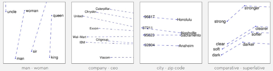
Text embeddings are a way to represent words or textual documents as large dimensional mathematical vectors, enabling computers—traditionally “dumb” in understanding language—to process text more effectively. They transform words into numerical vectors which capture their meaning based on their context. In this way, words that share similar meanings, context, or analogies are placed close together in the embedding space. Here’s a highly simplified example of how the words are represented and what counts as being close to each other.
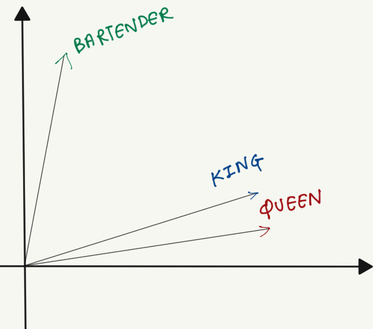
Here, the words “king” and “queen” are placed together in the space, whereas “bartender” is away from them, indicating no strong connection. While illustrations often show these embeddings in two dimensions, real-world embeddings commonly have up to 100 or more dimensions. Such high-dimensional spaces allow each vector component to represent distinct features of meaning.
Another key usage of these embeddings is to handle polysemic words, which are the same sounding/written words having different meanings depending on the context. For example, consider these two sentences:-
“I ate an apple.” vs. “Apple released a new phone this year.”
Here the word “apple” is being used in a different context. Text embeddings model these nuances, enabling more contextually accurate suggestions.
Understanding Languages - A Challenge for Eons
Understanding languages has always been a challenge. English itself is a very complex language—full of exceptions, contradictions, and rules that even we humans struggle to follow (after all, fish and ghoti can sound the same if you’re creative enough!). So, imagine how much more difficult it is for computers to make sense of human language and all its complexity. Well thankfully, innovation and hard work throughout the ages have brought us several techniques to make things work out, and that is exactly what you will be dealing with throughout this helpful blog. You will be looking at several models that help to transform textual data into different kinds of numerical representations because, after all, that is what our computers understand. You will also see how we can use this numerical data for tons of different use cases including suggestions of similar words!
Overview of the Models
Several models are employed to represent and process textual data. Some of the most well-known include:
- Bag of Words: It is the simplest form of text representation in numbers. Words are vectorized based on their count in the document or sample.
- TF-IDF: This algorithm works on the statistical principle of finding the word relevance in a document or a set of documents.
- Word2Vec: Words are vectorized, and these vectors capture information about the word's meaning based on the surrounding words. The word2vec algorithm estimates these representations by modeling text in a large corpus.
- GloVe: GloVe (Global Vector) is a model for distributed word representation where vector representations of words are obtained by mapping words into a meaningful space where the distance between words is related to semantic similarity.
The following sections provide a deeper look into these models, along with code snippets and examples.
Bag Of Words
The Bag-Of-Words model is a kind of representation that ignores word ordering and context but focuses on word multiplicity. Although sub-optimal, it is used in problems where word count can be used as a feature for solving the problem. The very first reference to this model can go back to 1954! It was published in an article by linguist Zellig Harris[1].
In the popular Bag Of Words Model, you vectorize words based on their count in the document or sample. Here’s how you can build a BOW:-
- You remove punctuations and lower the case.
- Then you eliminate the stopwords (words that are not meaningful for the suggestion, eg:- “and”, “or”, “the” etc.)
- After this, you create the count vector using different libraries, and then apply your models.
Now let’s see this in action, the corpus is a small set of search queries for buying electronics, the code below does the following:
- Data Preparation: The code starts by importing the necessary libraries. It then defines a list of sample search queries related to buying electronics.
- Text Preprocessing: Each query is converted to lowercase, split into individual words, and then cleaned of stopwords. Finally, it’s joined back into a processed string and appended to the corpus list.
- Vectorization with Bag of Words: The CountVectorizer() from sci-kit-learn transforms the cleaned text into a numerical matrix where each column represents a word, and each row represents a document (query). The values are the counts of how often each word appears.
- DataFrame Creation: This matrix is converted into a pandas DataFrame, making it easier to read and interpret. The DataFrame’s columns are the words, and each row corresponds to a processed search query.
- Output: Finally, the code prints the resulting table, providing a clear, human-readable representation of the Bag of Words features derived from the text.
import pandas as pd
from sklearn.feature_extraction.text import CountVectorizer
from nltk.corpus import stopwords
import nltk
search_queries = [ "buy a laptop online","cheap laptops for sale","best gaming laptop","online shopping for electronics", "buy smartphone online","cheap mobile phones","best budget smartphone","latest smartphone models", "buy books online","top books to read","best fantasy books" ]

corpus = [] #processing the corpus
for query in search_queries:
    review = query.lower()
    review = review.split()
    review = [word for word in review if word not in set(sw)]
    review = ' '.join(review)
    corpus.append(review)
##vectorization of BOW
vectorizer_bow = CountVectorizer()
X_bow = vectorizer_bow.fit_transform(corpus)
X_bow_dense = X_bow.toarray()
df_bow=
pd.DataFrame(X_bow_dense,columns=vectorizer_bow.get_feature_names_out()) df_bow.insert(0, 'Index', range(len(corpus)))
print("Bag of Words (BOW) Table:")
print(df_bow.to_string(index=False))
Output of the above code:
| Index | best | books | budget | buy | cheap | electronics | fantasy | gaming | laptop | laptops | latest | mobile | models | online | phones | read | sale | shopping | smartphone | top |
|---|---|---|---|---|---|---|---|---|---|---|---|---|---|---|---|---|---|---|---|---|
| 0 | 0 | 0 | 0 | 1 | 0 | 0 | 0 | 0 | 1 | 0 | 0 | 0 | 0 | 1 | 0 | 0 | 0 | 0 | 0 | 0 |
| 1 | 0 | 0 | 0 | 0 | 1 | 0 | 0 | 0 | 0 | 1 | 0 | 0 | 0 | 0 | 0 | 0 | 1 | 0 | 0 | 0 |
| 2 | 1 | 0 | 0 | 0 | 0 | 0 | 0 | 1 | 1 | 0 | 0 | 0 | 0 | 0 | 0 | 0 | 0 | 0 | 0 | 0 |
| 3 | 0 | 0 | 0 | 0 | 0 | 1 | 0 | 0 | 0 | 0 | 0 | 0 | 0 | 1 | 0 | 0 | 0 | 1 | 0 | 0 |
| 4 | 0 | 0 | 0 | 1 | 0 | 0 | 0 | 0 | 0 | 0 | 0 | 0 | 0 | 1 | 0 | 0 | 0 | 0 | 1 | 0 |
| 5 | 0 | 0 | 0 | 0 | 1 | 0 | 0 | 0 | 0 | 0 | 0 | 1 | 0 | 0 | 1 | 0 | 0 | 0 | 0 | 0 |
| 6 | 1 | 0 | 1 | 0 | 0 | 0 | 0 | 0 | 0 | 0 | 0 | 0 | 0 | 0 | 0 | 0 | 0 | 0 | 1 | 0 |
| 7 | 0 | 0 | 0 | 0 | 0 | 0 | 0 | 0 | 0 | 0 | 1 | 0 | 1 | 0 | 0 | 0 | 0 | 0 | 1 | 0 |
| 8 | 0 | 1 | 0 | 1 | 0 | 0 | 0 | 0 | 0 | 0 | 0 | 0 | 0 | 1 | 0 | 0 | 0 | 0 | 0 | 0 |
| 9 | 0 | 1 | 0 | 0 | 0 | 0 | 0 | 0 | 0 | 0 | 0 | 0 | 0 | 0 | 0 | 1 | 0 | 0 | 0 | 1 |
| 10 | 1 | 1 | 0 | 0 | 0 | 0 | 1 | 0 | 0 | 0 | 0 | 0 | 0 | 0 | 0 | 0 | 0 | 0 | 0 | 0 |
This results in a matrix of word counts, highlighting the importance of various terms across documents. Although simple, BoW can be a stepping stone to more sophisticated models.
Term Frequency - Inverse Document Frequency (TF-IDF)
TF-IDF weighs the importance of words more cleverly than BoW. This algorithm works on the statistical principle of finding the relevance of the word in a document or a set of documents.
The term frequency (TF) score measures the frequency of a word occurring in the document while the inverse document frequency (IDF) measures the rarity of the words in the corpus. It is given more mathematical importance as some words rarely occurring in the text still might hold relevant information.
Now let’s see the expressions that are used to calculate the tf-idf score:
where,
Here’s the representation through a code snippet, the code does the following:
- Vectorization with TF-IDF: TfidfVectorizer computes term frequency-inverse document frequency scores for each word in each document.
- Term Importance: TF-IDF highlights words that are important to a particular query but uncommon in the overall corpus, providing a more meaningful measure than raw counts.
- Data Representation: The resulting matrix is converted into a DataFrame, making it easy to see which words are most “informative” across all search queries.
##tf-idf representation
from sklearn.feature_extraction.text import TfidfVectorizer
vectorizer_tfidf = TfidfVectorizer()
X_tfidf = vectorizer_tfidf.fit_transform(corpus)
X_tfidf_dense = X_tfidf.toarray()
df_tfidf=pd.DataFrame(X_tfidf_dense,columns=vectorizer_tfidf.get_feature_names_out()) df_tfidf.insert(0, 'Index', range(len(corpus)))
print("\nTF-IDF Table:")
print(df_tfidf.to_string(index=False))
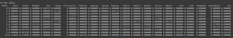
The above snippet of code converts our corpus into a TF-IDF representation, which measures the importance of words in each document relative to the entire corpus. Using TfidfVectorizer from the sklearn library, it computes the TF-IDF values for all words, transforms the data into a dense array, and organizes it into a dataframe for better readability. The final table shows each word's relevance across the documents, making it useful for text analysis tasks like identifying significant terms in a dataset.
TF-IDF Table:
Issues with the traditional models
While BoW and TF-IDF are important building blocks, they have limitations. They rely heavily on frequency, do not consider word order, and often produce sparse, high-dimensional representations that are computationally expensive. These models fail to capture nuanced semantic relationships or contextual meanings.
This is where Text embedding shines, models such as Word2Vec, GLoVe, and BERT, represent words as dense high-dimensional vectors. This way, similar words can be represented closer to each other and the context of the words is captured. For example, the words “happy” and “joyful” are closer in the embedding space. Also, the word order is preserved. Sentences such as “The man bit the dog” vs “The dog bit the man” are interpreted differently, while the earlier models would capture no difference between them.
We'll now walk through two of the most popular and highly advanced models, Word2Vec and GloVe.
Word2Vec
The Word2Vec model, developed by Google in 2013, is a highly influential machine learning model widely used in Natural Language Processing (NLP). It learns vector representations of words such that words with similar meanings appear close to each other in the vector space. Two primary methods drive this learning process:
- Continuous Bag of Words (CBOW)
- Skip-gram
This approach is often summarized by the phrase: "You shall know a word by the company it keeps."
Continuous Bag Of Words (CBOW):
Here, instead of just using the count of each word, CBOW uses a sliding window to predict a target word based on its surrounding words (context). For example:
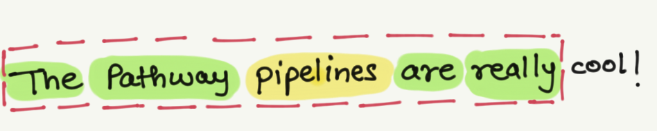
Here the word “pipelines” is the target word, whereas the other surrounding words provide the context.
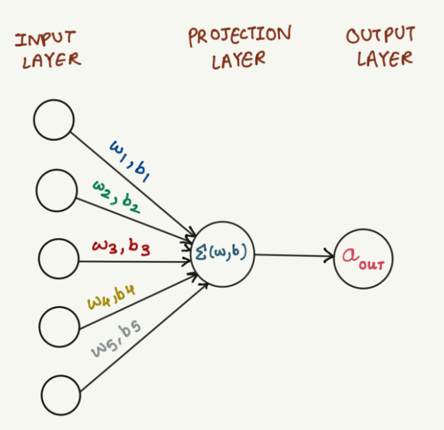
The CBOW uses a simple neural network to process the probabilities of the suggestion. This includes an input layer, a single fully connected hidden layer also known as the projection layer, and an output layer.
Here’s a simplified diagram of the neural network used by the CBOW method
Skip-gram This method works inversely to the CBOW, where the target word is known and the model tries to guess the context using it. It is more effective in identifying less frequent relationships and capturing more nuanced semantic patterns.
Here’s a diagram for the Skip-gram method:

Sample Code Using Word2Vec
import gensim.downloader as api
model = api.load("word2vec-google-news-300")

example_word = "computer"
similar_words = model.most_similar(example_word, topn=10)
print(f"Top 10 words similar to '{example_word}':")
for word, similarity in similar_words:
    print(f"{word}: {similarity:.4f}")
This code does the following:
- Pre-trained Model Loading: The code loads the pre-trained Google News Word2Vec model, which already has learned word meanings from a vast corpus of text.
- Semantic Similarity: most_similar() finds words closest in meaning to the example word “computer” by examining the vector space learned by the model.
- Output: The top 10 similar words and their similarity scores are printed, showcasing how Word2Vec captures semantic relationships rather than just word frequency.
Output of the above example:
Top 10 words similar to 'computer':
computers: 0.7979
laptop: 0.6640
laptop_computer: 0.6549
Computer: 0.6473
com_puter: 0.6082
technician_Leonard_Luchko: 0.5663
mainframes_minicomputers: 0.5618
laptop_computers: 0.5585
PC: 0.5540
maker_Dell_DELL.O: 0.5519

Global Representation of Vectors (GloVe)
The GloVe method, developed at Stanford University by Jeffrey Pennington and collaborators, is known as Global Vectors because it leverages the entire corpus’s global statistics. Unlike Word2Vec, which focuses on local context windows, GloVe constructs a co-occurrence matrix that measures how frequently pairs of words appear together. Using this global perspective, GloVe effectively captures both semantic and syntactic relationships, making it especially powerful for discovering word analogies.
Co-occurrence Matrix Example
Consider a small sample corpus:
corpus = [
"I like pathway","I like NLP","I enjoy pathway",
"deep learning is fun","NLP is amazing","pathway is fun"
]
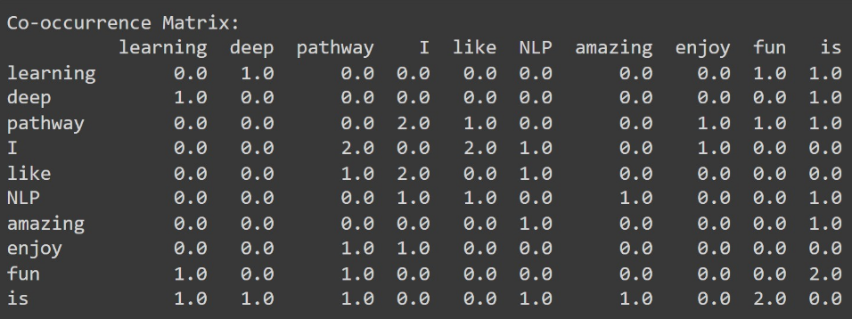
With a window size of 2, the model considers each target word and the two words surrounding it. This approach helps the model understand deeper relationships between words beyond simple frequency counts.
Sample Code Using GloVe
glove_file = 'glove.6B.100d.txt'
glove_model = load_glove_model(glove_file)
def find_similar_words(word, model, topn=10):
word_vector = model[word]
similarities = {}
for other_word, other_vector in model.items():
if other_word != word:
similarity = cosine_similarity([word_vector], [other_vector])[0][0]
similarities[other_word] = similarity
similar_words = sorted(similarities.items(), key=lambda item: item[1], reverse=True)[:topn]
return similar_words
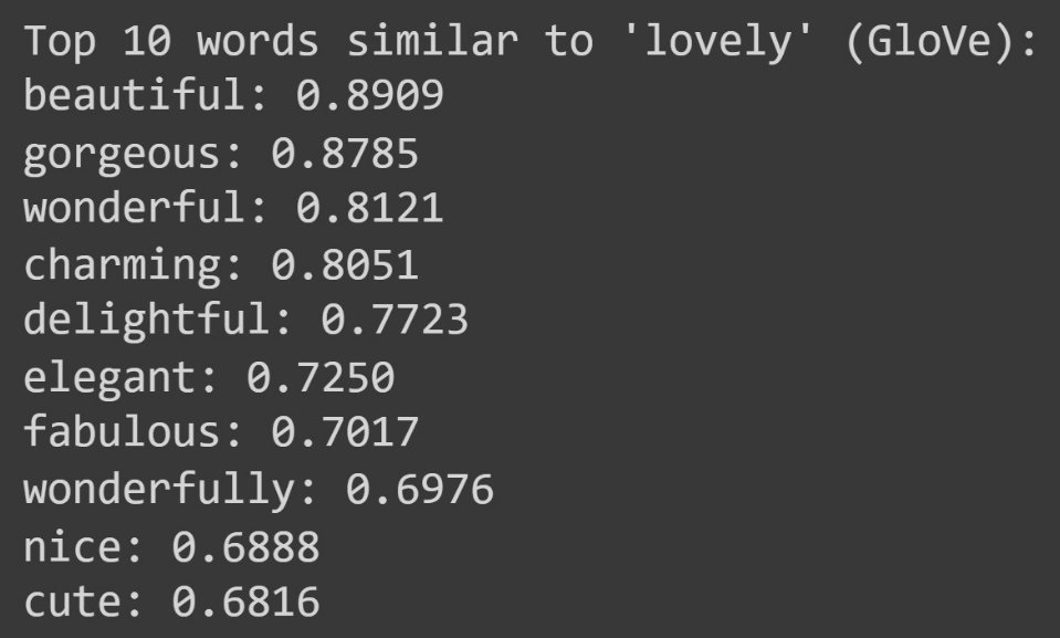
example_word = "lovely"
similar_words_glove = find_similar_words(example_word, glove_model, topn=10)
print(f"Top 10 words similar to '{example_word}' (GloVe):")
for word, similarity in similar_words_glove:
print(f"{word}: {similarity:.4f}")
Explanation:
- Loading the GloVe Model: The
glove.6B.100d.txtfile contains the pre-trained GloVe embeddings. The “6B” indicates it was trained on a dataset with 6 billion tokens, and “100d” means each word is represented by a 100-dimensional vector. - Finding Similar Words: The
find_similar_words()function calculates the cosine similarity between the target word’s vector and every other word’s vector in the model, returning the top matches. - Global Context: Unlike frequency-based models, GloVe embeddings capture both local context and global statistical properties, enabling more nuanced relationships to emerge.
Output:
How text embeddings capture analogies
Let us now try to understand how Text Embeddings capture the contextual relationships between countries and their capitals or verbs and tenses using GloVe embeddings, t-SNE, and PCA for visualization. As you've already looked through GloVe before, let us go over t-SNE and PCA in the following sections.
Dimensionality Reduction Techniques for Visualization
t-SNE (t-distributed Stochastic Neighbor Embedding)
t-SNE, short for t-distributed Stochastic Neighbor Emulation, is an unsupervised Machine Learning algorithm for dimensionality reduction ideal for visualizing high-dimensional data. It was developed in 2008 by Laurens van der Maaten and Geoffery Hinton. The process involves embedding high-dimensional points in low dimensions so that data loss is to a minimum. It preserves similarities between points as Nearby points in the high-dimensional space correspond to nearby embedded low-dimensional points. The same applies to distant points.
PCA (Principal Component Analysis)
The PCA unsupervised machine learning algorithm, which stands for Principal Component Analysis, was invented by the mathematician Karl Pearson in 1901. The following method also focuses on reducing dimensionality. Data in the high-dimensional space is mapped to data in the lower-dimensional space; the variance of the data in the lower-dimensional space should be the maximum. It is a statistical process that uses an orthogonal transformation and converts a set of correlated variables to a set of uncorrelated variables.
Now that you are well equipped with these powerful dimensionality reduction techniques, let’s move on to our fun analogies.
The fundamental approach of Text embedding is that you can represent words as vectors where every word can be expressed as a numerical vector in a high-dimensional space. Let's take the word 'king' for example. You can represent 'king' in an n-dimensional space where it will have n attributes. Words that appear in a similar context to 'king' will be closer to it in the embedding space. You can perform certain vector operations to reveal relationships between different words. The relationships can be shown as follows:
- Countries and Capitals: The interrelation between Paris and France is analogous to the interrelation between Berlin and Germany. Subtracting France from Paris isolates the concept of a "capital city" concerning a country. The relation between the four words in the vector space can be presented as follows:
vec(Paris) − vec(France)≈vec(Germany) - vec(Berlin)
Hence, you can say, '"Paris is to France as Berlin is to Germany". - Verb Tenses : Verb Tenses can also be shown similarly. You can consider "Walking is to Walked" as "Running is to Ran". In the vector space, it is represented as follows:
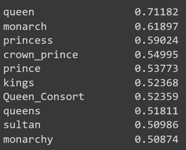
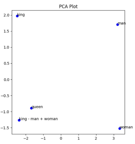
Walking – Walked ≈ Running – Ran - Gender Analogy: Construct a relationship between the words 'king' and 'queen'. In the embedding space, it can be expressed as follows:
vec(king)−vec(man)+vec(woman)≈vec(queen)
In the above expression, you can understand it as when you remove "man" from "king", it leaves a royal element, and when you add "woman", it becomes "queen".
- Gender Analogy Suggestions code:
import gensim.downloader as api model = api.load("word2vec-google-news-300") result = model.most_similar(positive=['king', 'woman'], negative=['man']) for i in result: print(f"{i[0]:<{20}} {i[1]:.6f}")` - Output:
- PCA Plots:
Evaluating models during production using RAG
The Internet is constantly flowing with an enormous amount of data, and our models need to keep up with it, constantly evolving according to the trends and information. One key technique to handle this is the Retrieval-Augmented-Generation (RAG). RAG is an AI framework that combines the strengths of traditional information retrieval systems (such as search and databases) with the capabilities of generative large language models (LLMs). The flow is as follows:-
- The user first enters a query, which is transformed into its embeddings to capture its semantic meaning.
- Documents are retrieved based on the embeddings, and then these docs, along with the embeddings are fed into a generative model.
- This helps to create a very contextual, efficient response, which is very much suited to the user.
Real-Time Embedding and Document Indexing with Pathway
While techniques like RAG help keep models dynamically updated with the latest data, effective deployment in production environments often demands robust, scalable solutions to manage continuous data streams and evolving embedding spaces. This is where Pathway comes in.
Pathway is a high-throughput, low-latency framework designed for building and deploying RAG-powered AI applications at scale. It offers a cloud-agnostic, container-based approach with over 350 data source connectors. It integrates YAML, Python, and SQL for flexible configuration and supports 300+ data connectors, including S3, Delta Lake, Iceberg, Kafka, NATS, and SharePoint.
The following example demonstrates how Pathway’s pipeline handles document ingestion, parsing, splitting, embedding, and indexing in real time. As soon as a new file is detected in the specified data source (here, a local folder with mode="streaming"), Pathway automatically re-runs the necessary steps to incorporate that file into the semantic index—no manual re-running of embeddings or re-indexing required.
Setup and Installations
If you are using Pathway locally, you will need to install Pathway LLM xpack with:
!pip install "pathway[all]"
Data Folder Setup: Creates a local directory named data/ where we will store and read our documents.
!mkdir -p 'data/'
import os

import json
from typing import Iterable, Literal, List
from pydantic import BaseModel, Field

# needed for the OpenAI embedder and the LLM we will use below, you can change the embedding provider, see the documentation:
# https://pathway.com/developers/api-docs/pathway-xpacks-llm/embedders
os.environ["OPENAI_API_KEY"] = "sk-"
Importing a Sample PDF File
!wget -q -P ./data/ https://github.com/pathwaycom/llm-app/raw/main/examples/pipelines/demo-question-answering/data/IdeanomicsInc_20160330_10-K_EX-10.26_9512211_EX-10.26_Content%20License%20Agreement.pdf
Pathway Imports and Pipeline Setup
- Imports: We import Pathway’s standard libraries and LLM toolkits.
- Reading in Streaming Mode: Notice the
mode="streaming"parameter inpw.io.fs.read().
This tells Pathway to watch the./datafolder for any file changes in real time. - Document Processing:
- Parser: Converts raw document files into text.
- Text Splitter: Splits text into manageable chunks before embedding.
- Embedder: Uses the OpenAI embedding model to transform text chunks into numerical vectors.
- Vector Index: A brute-force KNN factory that indexes embeddings to allow fast semantic search.
- DocumentStore: Orchestrates the entire ingestion pipeline (reading, parsing, splitting, embedding, indexing).
Whenever new files appear in thedata/folder, DocumentStore automatically processes them and re-runs the embedding/indexing pipeline in real time. - RAG App: A simple RAG (Retrieval-Augmented Generation) solution is configured with a GPT-based LLM and a top-k search for retrieved chunks.
import os
import getpass
import pathway as pw

from pathway.stdlib.indexing import BruteForceKnnFactory
from pathway.udfs import DiskCache
from pathway.xpacks.llm import embedders, llms, parsers, splitters
from pathway.xpacks.llm.document_store import DocumentStore
from pathway.xpacks.llm.question_answering import BaseRAGQuestionAnswerer, RAGClient
from pathway.xpacks.llm.servers import QASummaryRestServer


# read the text files under the data folder, we can also read from Google Drive, Sharepoint, etc.
# See connectors documentation: https://pathway.com/developers/user-guide/connect/pathway-connectors to learn more
folder = pw.io.fs.read(
    "./data",
    format="binary",
    with_metadata=True,
    mode="streaming"
)

# list of data sources to be indexed
sources = [folder]

# define the document processing steps
parser = parsers.UnstructuredParser()

text_splitter = splitters.TokenCountSplitter(min_tokens=150, max_tokens=450)

embedder = embedders.OpenAIEmbedder(cache_strategy=DiskCache())

index = BruteForceKnnFactory(embedder=embedder)

llm = llms.OpenAIChat(model="gpt-4o", cache_strategy=DiskCache())

document_store = DocumentStore(
    docs=sources, parser=parser, splitter=text_splitter, retriever_factory=index
)

# create the RAG app that will power the index, and serve the agent endpoint
rag_app = BaseRAGQuestionAnswerer(
    llm=llm,
    indexer=document_store,
    search_topk=8,  # number of retrieved chunks for RAG
)
Starting the Pathway RAG Server
- RAG Server: We instantiate a REST server (QASummaryRestServer) that exposes endpoints for question answering.
- Parallel Process: We run the server in a separate process, making it easy to handle incoming queries asynchronously.
import multiprocessing

# host and port of the RAG app
pathway_host: str = "0.0.0.0"
pathway_port: int = 8000

server = QASummaryRestServer(pathway_host, pathway_port, rag_app)

server_process = multiprocessing.Process(target=server.run, kwargs=dict(threaded=False))

server_process.start()
Querying the Existing Document
- Client Setup: We create a
RAGClientto interface with our Pathway RAG server. - Listing Documents: We see which files are currently in the document store.
- Question-Answering: We then query the content of the newly ingested PDF. Pathway automatically used the parsed, split, and embedded chunks from that PDF to generate an answer.
from pathway.xpacks.llm.question_answering import RAGClient

pathway_client = RAGClient(pathway_host, pathway_port)
pathway_client.pw_list_documents()
pathway_client.pw_ai_answer("What are the terms and conditions of the contract?")
Ingesting a Second (New) File
- Adding a New Document: We add a second PDF to the same folder watched by Pathway.
- Automatic Re-indexing: As soon as the file appears in
./data/, Pathway automatically triggers the pipeline:- Parsing → Splitting → Embedding → Indexing.
- Listing Documents: You will see that both the original PDF and the newly added PDF show up.
- Question-Answering: We can now query specifically about the second file. Pathway fetches the relevant text chunks from the newly embedded content to generate an answer, all without needing to manually re-run the code.
!wget -q -P ./data/ https://github.com/pathwaycom/llm-app/raw/main/examples/pipelines/gpt_4o_multimodal_rag/data/20230203_alphabet_10K.pdf
pathway_client.pw_list_documents()
pathway_client.pw_ai_answer("What are the table of contents in 20230203_alphabet_10K.pdf?")
Scalability and Advantages
Pathway’s Real-Time Ingestion
- Automatic Updates: Whenever a document is modified or a new file is added, Pathway automatically reprocesses and re-embeds that data.
- Consistency: Your index always remains up to date without additional manual steps.
Key Benefits
- Seamless Data Integration: Connect to diverse data sources—file systems, Kafka, APIs, SharePoint, S3, PostgreSQL, Google Drive, and more.
- Real-Time Indexing: New files, content updates, and deletions are continuously processed.
- Advanced Search: Use semantic vectors, hybrid queries, and full-text search in-memory for fast retrieval.
- No Extra Infrastructure: Deploy Pathway with minimal overhead—no separate streaming or indexing clusters needed.
Conclusion
Text embeddings are a way to represent words or textual documents as large dimensional mathematical vectors. They transform words into numerical vectors which capture their meaning based on their context.
A walk through the blog is as follows:
- Bag of Words: vectorize words based on their count in the document or sample
- Term Frequency - Inverse Document Frequency (TF-IDF): measures the frequency of a word occurring in the document while the inverse document frequency (IDF) measures the rarity of the words in the corpus
- Word2Vec: learn word associations and place words with similar meanings close to each other in the vector space
- Continuous Bag Of Words (CBOW): picks a target word, and its surrounding words are the context
- Skip-gram: target word is known and the model tries to guess the context using it
- GloVe: constructs a co-occurrence matrix which is then used to capture the semantic relations between the words
Here's a quick comparison between the models based on their strengths, weaknesses and key use cases
| Model | Strengths | Weaknesses | Key Use Cases |
|---|---|---|---|
| Bag of Words | - Implementation is simple and very effective with small datasets | - Word order and context is ignored.- High-dimensional and sparse vectors if the vocabulary is large. | - Text classification tasks with small datasets.- Basic sentiment analysis. |
| TF-IDF | - Weighs words by importance (frequency) within the document.- Reduces the impact of common and less informative words. | - Ignores word order and semantic meaning.- High-dimensional vectors for large vocabularies. | - Document retrieval and ranking.- Keyword extraction can be done. |
| Word2Vec | - Captures semantic meaning and relationships between words.- Dense, non-sparse vectors.- Effective for similarity and analogy tasks. | - Training can be computationally heavy.- Requires large datasets for better quality. | - Semantic search.- Better Sentiment analysis.- Suggesting similar words. |
| GloVe | - Captures both global and local context effectively.- Dense, low-dimensional vectors.- Good for analogy and similarity tasks. | - Computationally intensive to train.- Requires substantial preprocessing and large corpora for effectiveness. | - Document classification.- Named entity recognition.- Similarity and analogy tasks. |
Traditional techniques for representing words, such as Bag of Words, fail to capture the precise meaning of words and their relationships with other words. Word Embeddings overcome this issue as they can capture the semantic relationships between words and group them. For example, a search like 'running shoes' will also surface results for 'athletic footwear'- ensuring better recognition of the meaning. In this blog, you saw how the text embeddings capture the analogies using simple examples like Countries and Capitals, Verb Tenses, and Gender Analogy. Now you know better how Text Embeddings work in hidden, plain sight!
Citations
- IBM's blog on embeddings
- Turing's blog on word embeddings
- Stanford University's Global Vector Representations
- Pathway's Repositories
Editors
- Saksham Goel - DevRel Engineer at Pathway
- Shlok Srivastava - Lead Engineer at Pine Labs


